In previous entries in this series, I have shown what network analysis is and how you can use network analysis in archaeology to better understand connections, for example between different sites. Network analysis results in the generation of tables of data and graphs. This output is the result of mathematical algorithms that are “unleashed” onto the data.
In order to better understand how network analysis works, we need to get technical and talk about the mathematics behind the algorithms that are used in software applications like GEPHI and ORA. Incidentally, an algorithm is a process or set of rules that a computer follows to perform calculations or solve problems.
Networks are an abstraction that help us understand a phenomenon. They imply flow, interaction, exchange, similarities and affinities, or social relations between the elements that you study; which aspect of the network you emphasize depends on the phenomenon that you are studying.
The algorithms, called “measures” in network analysis, allow us to study the role that each element of the network, from now on referred to as nodes, has in the flow, or to determine the general structure of the network. Each measure takes different parameters into consideration and focuses on a particular aspect of the single nodes or of the network as a whole. This will become clearer when we look at a few concrete examples.
Centrality measures
First, we must distinguish centrality and network measures. The first examines the single nodes, while the second examines the general structure of the network. There are measures that focus on the edges, too, but for now I will not deal with those.
Starting with the centrality measures, the basic one is referred to as degree centrality. In a nutshell, this measure takes into consideration how many direct connections each node establishes or, in other words, how many direct neighbours each node has in the graph.
The basic mathematical algorithm that degree centrality is based on is:
$$C_i^{DEG} = \sum_{j= 1}^{n}a_{ij}$$
This is summing all the links – \(a_{ij}\) represents the matrix – that go from the other nodes in the network, \(j = 1\) up to \(n\), to the node that you are examining, \(i\). If you think about the matrix, \(i\) is the row and \(j\) is the column, hence you take the row and sum the values that it has for each column.

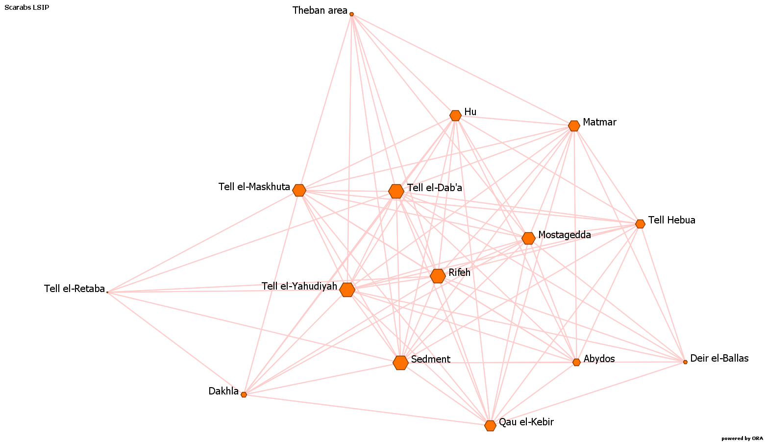
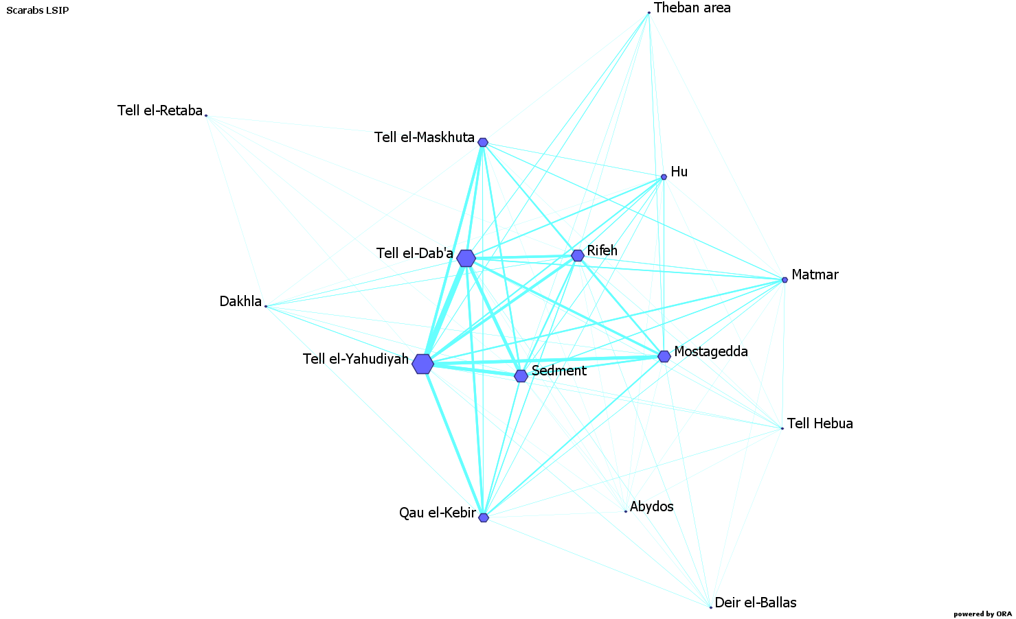
If you are calculating the degree of an undirected binary network, you basically count the links attached to each node (Fig. 1). If the network is weighted, then you also consider how strong the links are, i.e. of how many similarities or features in common it consists (Fig. 2).
If the network is directed, binary or weighted, it gets slightly more complicated: you need to take into account if the links start from the node, or if the node receives them. Therefore, you have an out-degree that counts the former, and an in-degree that counts the latter.

Basically, you not only calculate the operation shown above, to obtain the out-degree, but you reverse it and for each column you sum the values that it has for each row, to know the in-degree. You can then combine the two and also calculate the total degree.
Practical application
How can you apply this to an actual network? This depends on the field you are in and on what you study. For example, if you are studying a specific community – say, a village or the students of a school – it can tell you which individuals know more people.
If you are studying flight traffic, with a directed type of network, you can determine, for example, which airports receive more traffic. In archaeology, it also depends on your data. If you know the source of an object, or of a material resource, and you have enough data, you could, for example, make a directed network where you follow the path of the objects or of the material resources, and see how many types are sent from a site to the others.
In my case, studying objects from Egypt’s Second Intermediate Period (1775-1550 BC), I had to work with limited data: I only knew where the types of objects and the material resources I was studying have been found. I could not input any direction from where the types and material resources had reached their ultimate findspot.
The only factor that helped in this regard is that some of the material resources (e.g. amethyst, Jasper, haematite) are known to come from particular areas of Egypt. However, I did not have enough data to reconstruct the different stops that these materials made on their way to their findspots. What, then, did I examine and how did the degree centrality help?

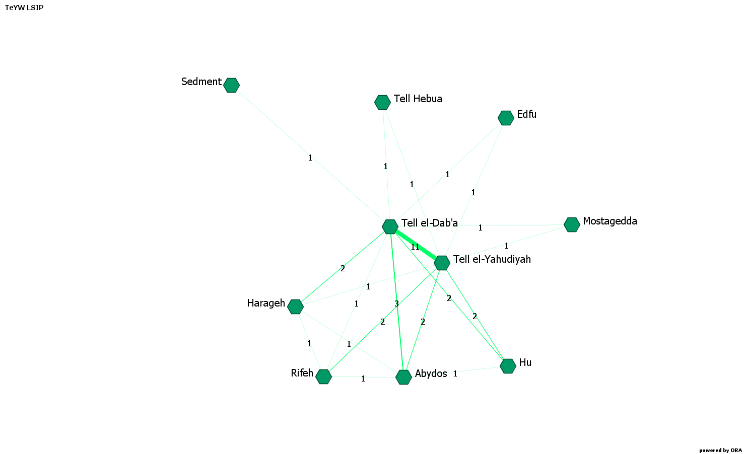
Mostly, what I focused on was the similarity of the material culture between different sites; hence my network was based on similarities. In my one-mode, weighted and undirected, network (Fig. 3), the degree centrality of a site was based on two factors: the number of sites with which the examined site shared particular types of objects, and the amount of the types of objects they had in common.
Thus, this measure indicated which sites had more objects in common with the larger number of sites and, as a consequence, had the stronger connections and were, therefore, more prominent. What did this prominence mean? Did it imply a special role in the distribution, the flow, or even the production, of these types, or even of the object themselves? This was the next question, which I answered by comparing the results of the degree centrality with other measures, and with what is known about the period from material remains and texts.
Structure of the network
A few measures based on the degree centrality are useful to analyse the structure of the network.
The first one is the degree distribution, \({P_{deg} (k)}\), where \(k\) is the degree centrality. To put it simply, you count how many nodes have a determined degree centrality in a network. For example, \({P_{deg} (13)} = 13\) means that in a network 13 nodes have degree centrality 3.
You could take this further and calculate k-cores, which are subnetworks (i.e. parts of a network) where the nodes have at least a certain degree centrality. However, here we go to more advanced operations, where you need to establish your own parameters for the calculations. Perhaps in a future article, I will discuss k-cores, together with m-slices.
The second measure is the average degree of all the nodes of the same network, which indicate the structural cohesion of the network represented in a graph.
The mathematical formula is as follows:
$$\bar{k} = \frac{\sum_i k_i}{n}$$
Basically, you sum – \(\sum_i\) – the degree centralities \(k_i\) of all the nodes, then divide this sum – that is, \({\sum_i k_i}\) – by the number of nodes, \(n\). The advantage of this measure is that it does not depend on the size, i.e. the numbers of nodes in a network, but on the degree centralities. Hence, it allows for easier comparison between networks of different sizes.
For example, when I analyzed the types of objects that the sites in Egypt have in common during the Second Intermediate Period, this measure could have been useful if I wanted to compare the network created by the types of beads with the network created by the types of stone vessels.
Lastly, a more advanced measure that you can use to determine the inequality of how the nodes are connected is the degree variance. It derives from the average degree, which is the average squared deviation between the degree of each node and the average degree.
Mathematically, it looks like this:
$$\mathcal{v}(G) = \frac{\sum_i (k_i - \bar{k})^2}{n}$$
To put it simply, you calculate the difference between the degree of each node \(k_i\) and the average degree, \(\bar{k}\) (vocalized as K-bar). Then, you square each of this number: \((k_i - \bar{k})^2\). In statistics, squaring when calculating deviation is done to avoid negative values in the calculation. Next, you sum all the numbers obtained: \(\sum_i\), etc. This sum is then divided by the number of nodes in the network, expressed as \(n\).
Closing remarks
I may discuss other measures in future articles. But at this point, I would like to emphasize that you should not be discouraged by the mathematics involved. Even though there are many concepts involved form various fields of mathematics (e.g. statistics, trigonometry, calculus, graph theory), nobody will ask you to become a mathematician.
What is important, however, is that you have an understanding of the formulas and of what they mean, so that you can interpret your results more correctly. Once you grasp the mathematical aspects, you can come up with your own methodologies and create new mathematical models.
How to get there? As with everything, it is a matter of training. Read and try to get an insight into what other researchers have done. Search for yourself if you don’t know some of the mathematical symbols or concepts involved. In other words: be curious. Nowadays there are many resources available for free online, you just need to look for the information.
And don’t forget: if you find something too difficult, don’t be afraid to reach out to someone who has more experience in the matter. Bear in mind that it takes time: you will not achieve these insights overnight. Particularly at the beginning of your journey, you will come across many things you are not familiar with, depending on your personal background. But little by little, you will learn and be able to increase your knowledge until you can deal with the more complex aspects of network analysis.
Further reading
- J.M. Bolland, “Sorting out centrality. An analysis of the performance of four centrality models in real and simulated networks”, Social Networks 10 (1988), pp. 233-253.
- S.P. Borgatti, “Centrality and network flow”, Social Networks 27 (2005), pp. 55-71.
- L.C. Freeman, “Centrality in social networks. Conceptual clarification”, Social Networks 1, pp. 215-239.
- J. Scott, Social Network Analysis (fourth edition, 2017).
The mathematical formulae were taken from this website by Omar Lizardo and Isaac Jilbert. The mathematics were formatted in LaTeX and are rendered on this page using MathJax, a JavaScript display engine.
