
In the previous articles in this series, I have discussed the three main centrality measures used in network analysis. I have shown how you can calculate and interpret the degree centrality, the betweenness centrality, and the closeness centrality, as well as other algorithms based on them.
To recap, the degree centrality counts an entity’s number of links, the betweenness centrality calculates how often an entity is in the path linking other two entities, and the closeness centrality is based on how long the paths connecting an entity with the others are. All these features are considered what makes a node central or prominent in a network.
In this article, I focus on the eigenvector centrality, which is the last of the four main measures used in network analysis. This measure indicates how important an entity is, based on how important the entities in contact with it are. In other words, the eigenvector centrality reveals which entities are better connected to important entities in the network.
It doesn’t matter how many connections an entity establishes, like the degree centrality, or what “linking power” these connections have, like betweenness centrality, or how easy they make to reach (or be reached by) others, as in the closeness centrality. What matters is the importance of the other entities connected to the entity that you are studying. It is not about the quantity, but the quality of the connections: “few but good”, as you would say.
Matrix multiplication
The eigenvector centrality is based on the eigenvalue, meaning that the value of an entity is based in the value of the entities connected to it: the higher the latter is, the higher the former becomes. What is this value, and what does it is meant by important entities, mentioned above?
In the simplest case, this means the entities with the highest degree centrality. You could modify your calculations and consider other aspects, if needed for more complex studies. How you can do that will be clear by the end of the article.
For now, the point here is that the eigenvector centrality is based on the value of an entity’s neighbour(s), and not on an intrinsic value of the entity itself (like the number or length of its connections). Therefore, the eigenvector centrality can be considered a special case or generalization of the other three main centrality measures (degree, betweenness, closeness).
Going to the more mathematical aspect, let’s start how to practically find the eigenvalue. However, before continuing it is necessary to know how a matrix multiplication works.
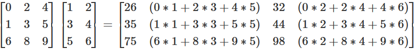
As you can see in the figure above, you take each number from each row of the first matrix (matrix A), and separately multiply it by each value of each column of the second matrix (matrix B), and then sum the results. You start with the first row of matrix A, take the first number and multiply it by the first number of the first column of matrix B, then you take the second number of the same row and multiply it by the second number of the same column, and so on until you have finished all the numbers in the row and the column, then sum the results of these multiplications: this will be the number in the first row and in the first column of matrix C.
So the first number of the results (matrix C) is \(26\), because you go through each of the numbers of the first row of matrix A and multiply these with the values in the column of matrix B. Hence, you arrive at this number as follows: \(0*1+2*3+4*5\). time you take the values of the second column of the second array: \(0*2+2*4+4*6\) results in \(32\).
Then, you do the same steps with the same row from matrix A, but the second column of matrix B: this will be the number in the first row and in the second column of matric C. You continue until you have multiplied the first row of matrix A by each column of matrix B, so that the first row of matrix C is complete. For the second column result in the first row of the third matrix, you do the same as before, but this
Afetrwards, you start the same process with the second row of matrix A, multiplying it by each column of matrix B like explained: this time the results will go in the second row of matrix C. You do this until you have completed all the rows of matrix A: matrix C should have the same number of rows as matrix A and the same number of columns as matrix B.
It is, technically speaking, a dot product, which is used in vector calculations: matrices can, and this is useful to do, thought of as vectors. From the same reasoning it also derives that, to multiplicate two matrices, one condition needs to be met: the numbers of columns in the first matrix needs to be the same as the number of rows in the second matrix.
You can also see how, contrarily to algebraic multiplications, matrix multiplication (and in general dot product) is not commutative: inverting the order of the matrices will give a different result.
The eigenvector centrality
We can now get on with the eigenvector centrality. You can follow all the described steps in the figure below:
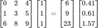
The first matrix above is matrix A, shown also in the previous section; the matrices after the equals sign are matrix D and matrix E. The normalized value of matrix D is \(14.67\).
As I mentioned, in the simplest case you can use the degree centrality as the starting point of your eigenvalue. But, instead of using the calculation showed in the relevant article, you need to find it out by multiplying the matrix by a column of all 1. This is the same as simply summing the values of each row, which is basically how to find out the degree centrality directly from the matrix.
Let’s take again matrix A, and multiply by such a column. This will give you a one-column matrix, matrix D, where each row corresponds to the degree centrality of each entity in your starting matrix. The next useful step is to find the normalized value of the degree centrality: you sum the square of the numbers of matrix D, divide it by the amount of its rows, and make a square root of the result. Afterwards, you divide each number in matrix D by the normalized value. This will give you a new one-column matrix, matrix E, where each row shows the eigenvector of each entity in the rows of your starting matrix.
This eigenvector is based on the value of the immediate neighbours of each entity, i.e. the ones with which it shares a link. You can reiterate this process, to include also the value of the second-degree neighbours, i.e. immediate neighbours of the immediate neighbours of each entity. This is shown below:
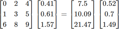
The first matrix is matrix A, the second is matrix E, the third (after the equals sign) is matrix F, with a normalized value of \(14.36\), and the final matrix is matrix G.
This time, instead of multiplying your starting matrix by a column of all 1, you multiply it by matrix E, obtaining matrix F. You can then reiterate again, as you can see in the formula below:
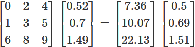
The first matrix is A, the second G, the third (after the equals sign) is matrix H, with a normalized value of \(14.67\), and the final matrix is I.
Initially multiply your starting matrix (i.e. matrix A) by matrix G (the second one), which is the result of the previous reiteration; this way, you include the value of the third-degree neighbours – you guessed it: neighbours of neighbours of neighbours – in the calculations.
You can keep reiterating the process to include up to the furthest degree of separation present in the network. How do you know you have reached the maximum amount of reiteration? A rule of thumb is that the normalized value in the new reiteration starts being very similar to the one in the previous reiteration(s); in other words, the unit and the first decimal (or the first two, or even more, depending on the approximation you opt for) remain the same.
The calculations described start by multiplying the starting matrix by a column of 1, as in the last figure. You can also say that the matrix was multiplied by a scalar of one. Multiplying a row by a scalar, basically a single value of your choice or dictated by your research, works exactly as multiplying it by a column of all same number (like a column of all 1, like matrix D).
The result in the figure was a one-column matrix with values corresponding to the degree centrality. However, you could choose to start with other scalars, depending on your research. Furthermore, you could choose to not normalize the value of matrix D, and simply keep reiterating by multiplying the starting matrix by the product of your previous multiplication.
The point is, that at the end you will have a value for each entity in your matrix, which tells you how important his connections are, for example which entity is connected to entities with the highest degree centrality. It can be understood how an entity that itself has a high degree centrality, or a high betweenness centrality, or a high closeness centrality, will not necessarily have a high eigenvector centrality.
For example, if an entity A is connected to many other entities, but these other entities are themselves peripheral and not further connected to others, entity A will have a high degree centrality, but a low eigenvector centrality. Therefore, an entity with a high eigenvector centrality is connected to prominent/popular/important entities in the network (the definition of it depending on your research) and, even though is itself not popular, can exploit the popularity and the influence of its connections.
In a human social network, for example, someone with a high eigenvector centrality is simply what is commonly known as someone with influential ties, which this someone can use to gain special treatment, protection, or other advantages, while others that do not share the same influential ties can’t. What influential means and what can be gained of course varies depending on the social context.
A practical example
There is a tendency for entities with a higher degree centrality to have also a higher eigenvector centrality, and vice versa, which I have noticed also when studying the networks based on the material culture in Egypt during the Second Intermediate Period, which can be noticed for example in figures 1 and 2.

In the case of my research, what did it mean when a site (which was the main entity in the matrix) had a higher or lower eigenvector centrality? More in general in archaeology, what can a higher or lower eigenvector centrality imply? It can mean that a site is in contact with another site that has many connections, which means that the community inhabiting or buried at a site could be in good contact with the community of a centre that was focal (because producing or receiving or (re)distributing) in the circulation of a particular type of object.
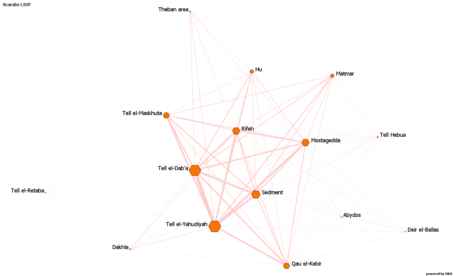
For example, in the netwrok based on the types of scarabs and seals in common between the Egyptian sites during the Late Second Intermediate Period, Tell el-Dab’a, Tell el-Yahudiyah and, on a lower degree, Tell el-Maskhuta, Sedment, Rifeh, Mostagedda, and Qau el-Kebir, had the highest eigenvector centrality, meaning that the communities present there were in contact with communities present at sites that were focal, in the meaning explained above, in the circulation of these designs.
In the case of Tell el-Dab’a, and probably Tell el-Yahudiyah, the site was a focal site itself, in the circulation of scarabs and seal design. The network was not directed, meaning that I could not see if the community at the focal site was importing or exporting these designs (or maybe a two-way influence and transmission?). However, the point was that a community in contact with one inhabiting a focal site had, through this, more possibilities and more “open doors” to get the product in or out, basically using the other one’s popularity.
Closing remarks
This concludes the overview on the main centrality measures and algorithms used in network analysis. There are more, such as e.g. Google’s Page rank, and I invite you to explore them and see what best fits your research, but these are often variations, or they take further the main measures discussed in these last four articles.
As always, don’t be scared of all the maths involved, as long as you grasp the basic and understand the true meaning behind it, you will be fine. And as previously said, take your time to investigate, learn and play around: it’s just part of the process.
In the next instalments of this series, I will discuss different types of matrices that you can create, other than the adjacency, and more about the different types of connections between entities in the graph (i.e. paths, walks, etc.), and strategies (like thresholds, tiers, ranks) that you could use to make sense of the results of the different algorithms.
If there is an interest, future articles will be also about measures and algorithms focusing on the edges and on the so-called “ego networks” (personal networks, centred on one entity and shaped according to its perspective and its personal ties). Until next time!